Analyzing Common C++ Performance Bottlenecks with Intel® VTune™ Profiler (Windows)

Use Cases and Prerequisites

This article shows how to use Intel® VTune™ Profiler on Windows to identify and analyze performance bottlenecks in serial and parallel applications. We use VTune’s built-in matrix sample matrix-multiplication application as the subject for analysis and optimization (note: because GitHub is used as the image host, some images load a bit slowly).

This article requires several Intel software tools. For convenience, you can download the Intel® oneAPI Base Toolkit directly:

• Intel® oneAPI Base Toolkit (Recommended)
• Standalone Intel® VTune™ Profiler
• Standalone Intel® oneAPI DPC++/C++ Compiler

PS: This article uses the Intel® oneAPI DPC++/C++ compiler to establish a common baseline for performance and performance gains. Depending on the compiler you use, the results and workflow may differ slightly. The VTune version used here is 2021; other versions may behave a little differently.

Workflow Overview

The article follows these steps to identify and fix the most significant performance issues in the sample matrix application:

1. Establish an application performance baseline
2. Identify the main bottleneck in the matrix application
3. Remove the memory-access bottleneck
4. Evaluate the performance improvement
5. Resolve the vectorization issue
6. Perform microarchitecture analysis
7. Visualize the performance gain

The detailed steps are described in the sections below.

Establishing a Performance Baseline

Run a Performance Snapshot

The first step in analyzing an application with VTune is to create a project. A project is a container that stores the analysis configuration and the collected results. VTune provides a preconfigured sample matrix project for use with the prebuilt matrix sample application.

First, open the preconfigured matrix project:

1. Start the VTune Profiler GUI.

   a. Run the following script to set the required environment variables:

   1install-dir\env\vars.bat
   

   PS: For VTune, the default install-dir is [Program Files]\Intel\oneAPI\vtune\version.

   b. Find the VTune Profiler icon in the Start menu and launch VTune Profiler.

   You may need to run VTune as administrator to use some analysis types.

2. The VTune welcome screen appears after the product starts.

The sample matrix project should already be open in the Project Navigator. If it is, no further action is needed. If the sample matrix project is not available in the Project Navigator, open it manually:

a. Click the Menu button, then choose Open -> Project… to open an existing project.

b. Browse to the project on your local machine and click Open.

By default, it is located in:

1[Users]\<user>\Documents\VTune\Projects\sample (matrix)

VTune opens the matrix project in the Project Navigator.

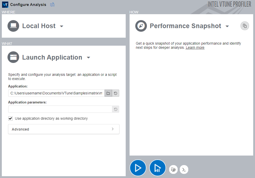
To start a performance snapshot analysis of the matrix sample application, do the following:

Click the Configure Analysis button to start a new analysis. The default analysis is preconfigured as Performance Snapshot for the local system’s matrix application. Then click Start to run the analysis, as shown below:

After letting it run for a while, click the pause/stop button. VTune will finalize the collected result and open the Summary view for the Performance Snapshot analysis.

Analyze the Performance Snapshot Result

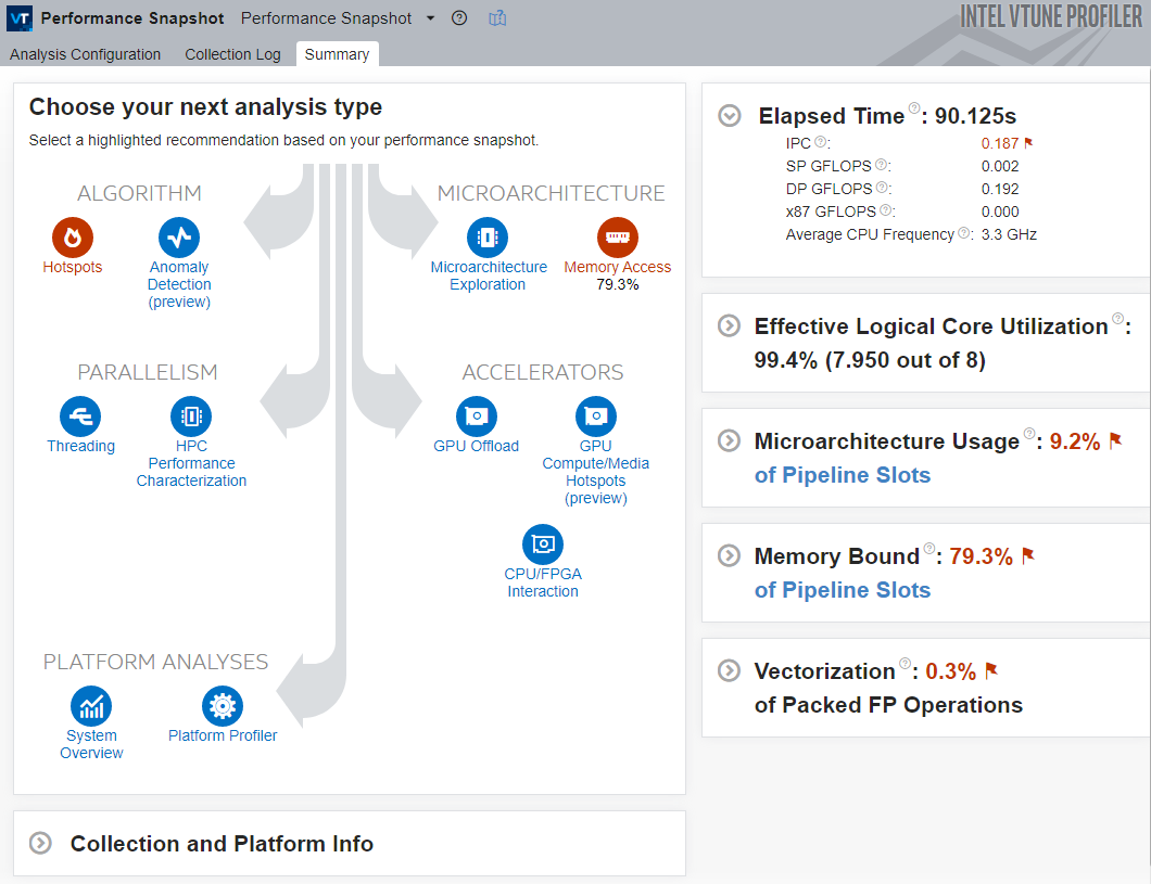
The Performance Snapshot Result Summary tab shows the following:

• Analysis tree: Performance Snapshot exposes additional analysis types that may help investigate the application’s performance issues in greater depth. Analysis types related to detected issues are highlighted in red.
• Metrics Panes: These panes show the high-level metrics that contribute most to the estimated application performance. Problem areas are highlighted in red. You can expand each pane to see more detail and lower-level metrics that help narrow down the cause.
• Collection and Platform Info: This pane shows information about the system used to collect this particular result. It is useful when opening results collected on other hardware platforms.

In this case, the following metrics stand out and point to the bottleneck:

1. The application’s Elapsed Time is very high.
2. The Memory Bound metric is high, which indicates a memory-access problem. Performance Snapshot therefore highlights memory-access analysis as a likely starting point and indicates that this bottleneck is the most severe and contributes the most to the total runtime.
3. For a modern superscalar processor, the IPC (instructions per cycle) value is very low, which shows that the processor is stalled most of the time.
4. Performance Snapshot highlights Hotspots as a good next step. In general, Hotspots is a good candidate for the first deep-dive analysis because it highlights hot code regions or the code that contributes most to runtime.

Next, start with Hotspots and see which code region in the matrix application has the largest impact on performance.

Analyzing the Application Bottleneck

Run Hotspots and Analyze

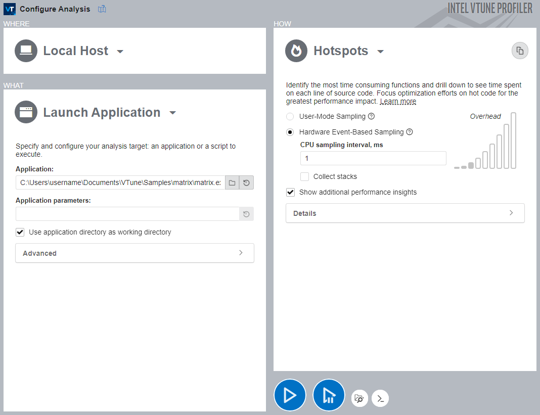
To run Hotspots from the Performance Snapshot summary window, do the following:

1. Click the Hotspots icon in the analysis tree to open the Configure Analysis window.
2. In the WHERE pane, select Local Host.
3. If you are using the provided sample matrix project, the WHAT pane should already be configured. If not, provide the application path in the Application text box.
4. In the HOW pane, Hotspots is already selected. For collection mode, you can choose between User-Mode Sampling and Hardware Event-Based Sampling. The methods differ, but in general, hardware-event-based sampling is preferred because it provides more detailed information with lower overhead.
5. Click Start to run the analysis.

After the sample application exits, VTune finalizes the result and opens the Summary view.

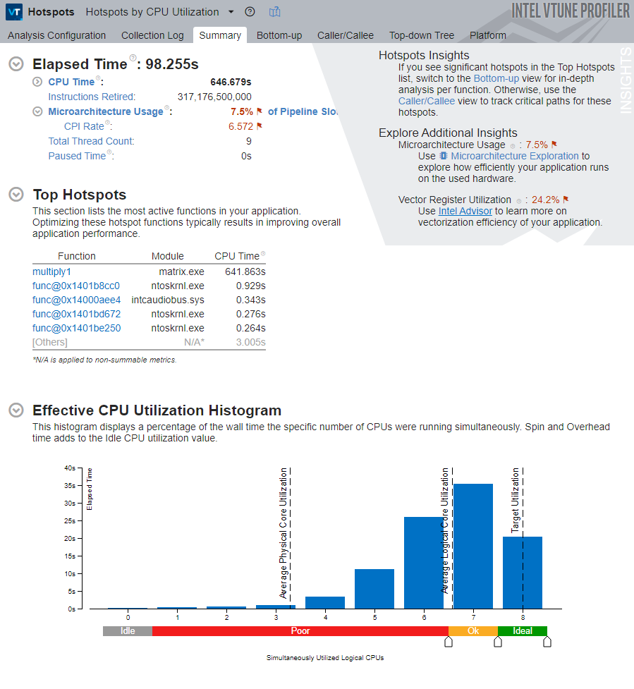
This view exposes several metrics. Hover over the question-mark icons to read the detailed descriptions of each metric.

Note that the application’s total CPU Time is about 642 seconds. This is the sum of CPU time across all threads. There are 9 threads in total, so the application is multithreaded.

The Top Hotspots section in the Summary window shows the most time-consuming functions, sorted by CPU time. For this sample, the multiply1 function takes about 640 seconds to execute, yet it still appears at the top of the list as the hottest function.

The Effective CPU Utilization Histogram below the Summary window shows the elapsed time and utilization levels of the available logical processors, and gives a visual indication of how many logical processors were used during execution. Ideally, the tallest bar in the chart should match the target utilization level.

To get a per-function view of the code, switch to the Bottom-up tab. By default, the data in the grid is grouped by function. You can change the grouping level using the Grouping menu at the top of the grid.

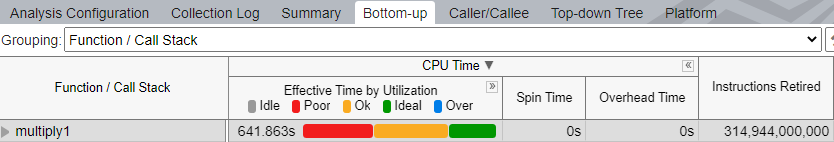
The multiply1 function takes the most time, about 640 seconds, and shows poor CPU utilization.

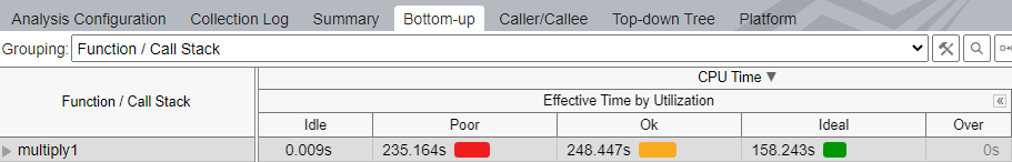
To inspect per-function CPU-utilization details, expand the Effective Time by Utilization column group using the expand button in the Bottom-up pane.

Double-click multiply1 in the Bottom-up grid to open the source window.

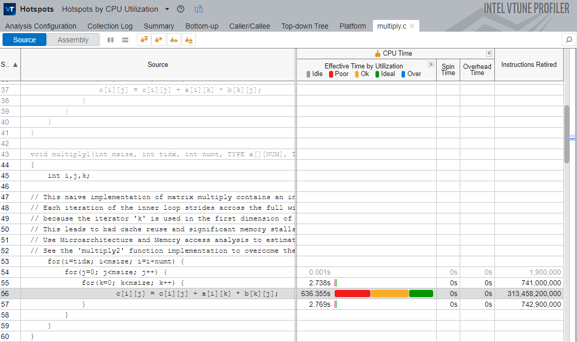
PS: If the target application is different, make sure it includes debug information and that the source path matches the debug info.

Note that the most time-consuming line is the loop that performs matrix multiplication inside multiply1. To analyze the memory behavior of this loop, run Memory Access next.

Run Memory Access and Analyze

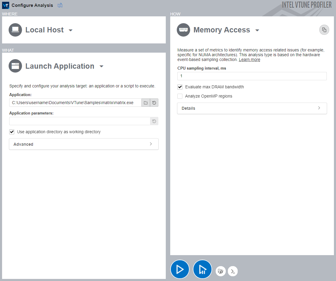
To run Memory Access analysis:

1. Click the Memory Access icon in the previously collected Performance Snapshot result, or click Configure Analysis in the main toolbar.
2. If you clicked the Memory Access icon, the analysis should already be selected. If not, select it in the HOW pane.
3. In the HOW pane, disable Analyze OpenMP regions because this application does not need it.
4. Click Start to run the analysis.

The result looks like this:

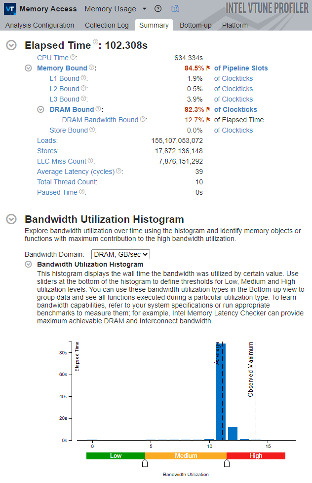
Again, the application is tightly constrained by memory access. The fact that the system is not limited by DRAM bandwidth alone indicates that the application is constrained by frequent but small memory requests rather than by saturated physical DRAM bandwidth.

Switch to the Bottom-up tab to inspect the exact metrics for multiply1:

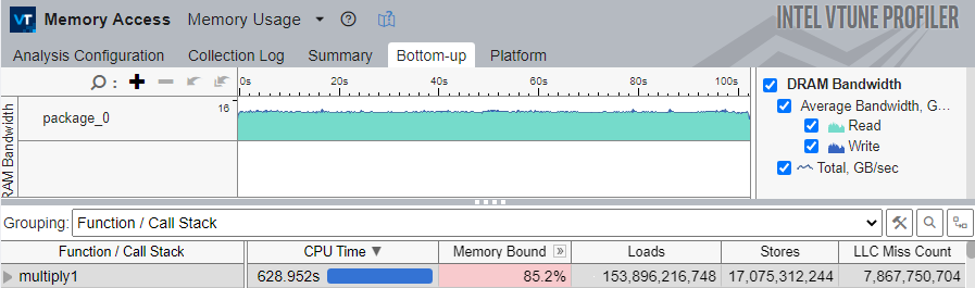
The multiply1 function is at the top of the grid, with the highest CPU time and a high memory-bound metric.

Note that the LLC Miss Count metric is very high. This indicates that the application uses a cache-unfriendly memory-access pattern, causing the processor to miss the LLC frequently and request data from DRAM, which is costly in terms of latency.

A good way to fix this is to apply loop interchange. In this case, loop interchange changes how matrix rows and columns are addressed in the main loop. That removes the inefficient memory-access pattern and lets the processor use the LLC more effectively.

Removing the Memory-Access Bottleneck

Use the Intel® oneAPI DPC++/C++ compiler to edit and rebuild the code in Microsoft Visual Studio as follows:

1. Find the matrix sample application folder on your computer. By default, it is located at: [Documents]\VTune\samples\matrix.
2. Open the matrix.sln Visual Studio solution in ..\matrix\vc15 inside that folder.
3. Make sure the Release configuration and x64 platform are enabled when building the application.
4. In Solution Explorer, right-click the matrix project and choose Properties.
5. Under Configuration Properties -> General, change Platform Toolset to Intel C++ Compiler version.
6. Under C/C++ -> General, make sure Debug Information Format is set to Program Database (/Zi).
7. Under C/C++ -> Optimization, make sure Optimization is set to Maximum Optimizations (Favor Size) (/O1).
8. Under C/C++ > Diagnostics [Intel C++], set Optimization Diagnostic Level to Level 2 (/Qopt-report:2).
9. In multiply.h, change line 36 as follows:

1- #define MULTIPLY multiply1
2+ #define MULTIPLY multiply2

This switches the program to the multiply2 function in multiply.c, which implements the loop interchange technique used to fix the memory-access problem. Finally, rebuild the application.

Evaluating the Performance Improvement

To see the improvement provided by loop interchange, run Performance Snapshot again:

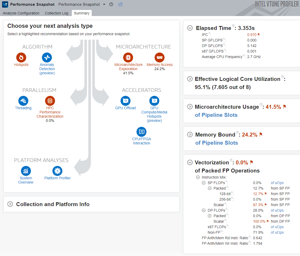
Observe the following key metrics:

• The application’s Elapsed Time decreases significantly. This improvement is mainly due to removing the memory-access bottleneck that caused the processor to miss cache frequently and fetch data from DRAM, which is very expensive in terms of latency.
• The Vectorization metric is 0.0%, which means the code is not vectorized. Therefore, Performance Snapshot highlights HPC Performance Characterization as the next likely step.

In this case, the code is not vectorized because the Intel® oneAPI DPC++/C++ compiler does not perform vectorization when compiling with the preferred binary-size optimization level (/O1).

To enable automatic vectorization in the compiler through Visual Studio, follow these steps:

1. Right-click the matrix project and choose Properties.
2. Under C/C++ > Optimization, set Optimization to Maximum Optimization (Favor Speed) (/O2).
3. Save the configuration changes and rebuild the application.

Solving the Vectorization Problem

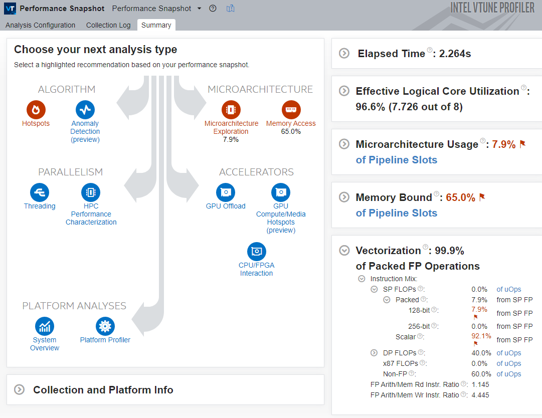
After recompiling the application with /O2, run Performance Snapshot again to analyze vectorization efficiency:

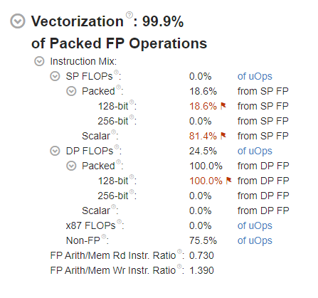
Observe the following key metrics:

1. The overall Vectorization metric is 99.9%, which means the code has been vectorized.
2. However, there is a warning flag next to 128-bit Packed FLOPs. Hover over the red flag icon or the metric value to see the issue description.

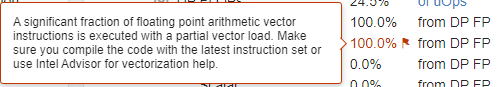
In this case, VTune indicates that a large portion of the floating-point instructions are executed under partial vector load.

Because the analysis was run on a machine with an Intel processor capable of using the AVX2 instruction set, all instructions were executed with only 128-bit registers, which means the 256-bit-wide AVX2 registers were not used at all. VTune therefore flags 100.0% utilization of the 128-bit vector registers as a problem.

To see which vector instruction set is actually used, run HPC Performance Characterization:

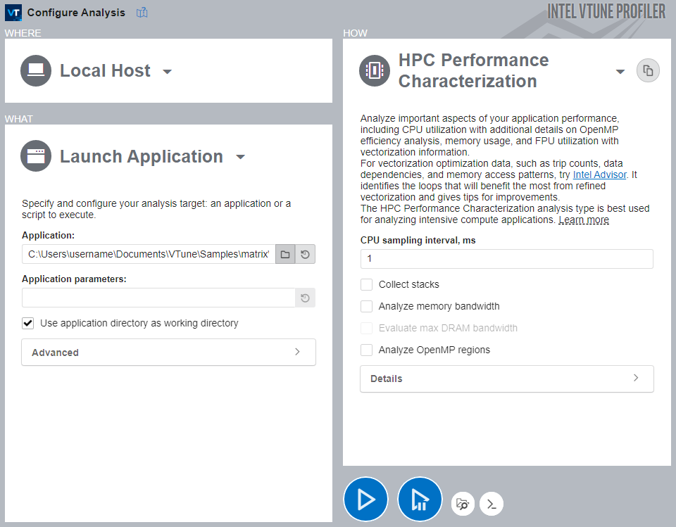
To run the analysis:

1. Click the HPC Performance Characterization icon in the analysis tree.
2. Disable Collect stacks, Analyze Memory bandwidth, and Analyze OpenMP regions because they are not needed for vectorization analysis.
3. Click Start to run the analysis.

After data collection completes, VTune opens the default summary window for HPC Performance Characterization:

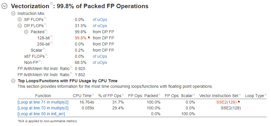
Focus on the Vectorization section in the Summary window.

Note that the main loop in multiply2 is vectorized with the older SSE2 instruction set, while compilation and analysis were performed on a processor that supports AVX2. As a result, some hardware resources are still underutilized.

To use the vector instruction set that is best suited to the platform, one possible approach is to tell the compiler to use the same vector extension that is best available on the processor where the compilation is being performed.

Follow these steps to enable platform-specific vectorization in Visual Studio:

1. In the Solution Explorer pane, right-click the matrix project and choose Properties.
2. Go to C/C++ > Code Generation [Intel C++].
3. Set Intel Processor-Specific Optimization to Same as the host processor performing the compilation (/QxHost) so that the compiler uses the best instruction-set extension available on the processor running the build.
4. Save the changes and rebuild the application.

Run Performance Snapshot again to confirm that the application is properly vectorized.

Observe the following key metrics:

1. The application’s Elapsed Time decreases slightly.
2. The Vectorization metric is 99.9%, so the code is fully vectorized.
3. A total of 100.0% of the Packed DP FLOP instructions are executed with 256-bit registers. Even without running HPC Performance Characterization, this shows that the AVX2 vector extension is fully utilized.
4. VTune also highlights microarchitecture-utilization metrics and suggests Microarchitecture Exploration to understand exactly where the application is underutilizing the microarchitecture.

Performing Microarchitecture Analysis

Although the earlier optimizations greatly reduced total runtime, there is still room for improvement. Performance Snapshot shows that the microarchitecture is not being used very efficiently.

Run Microarchitecture Exploration to identify opportunities for improvement.

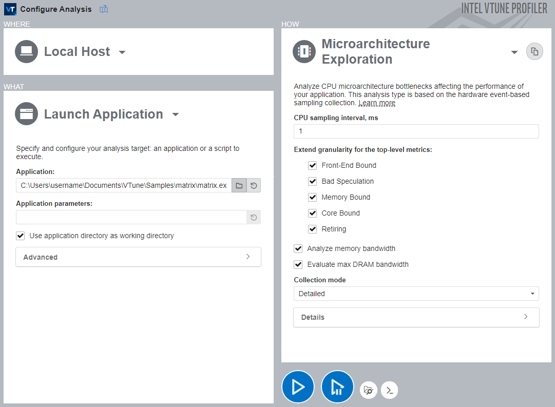
To run Microarchitecture Exploration:

1. In the Performance Snapshot analysis tree, click the Microarchitecture Exploration icon.
2. In the HOW pane, enable all additional options.
3. Click Start to run the analysis.

The result looks like this:

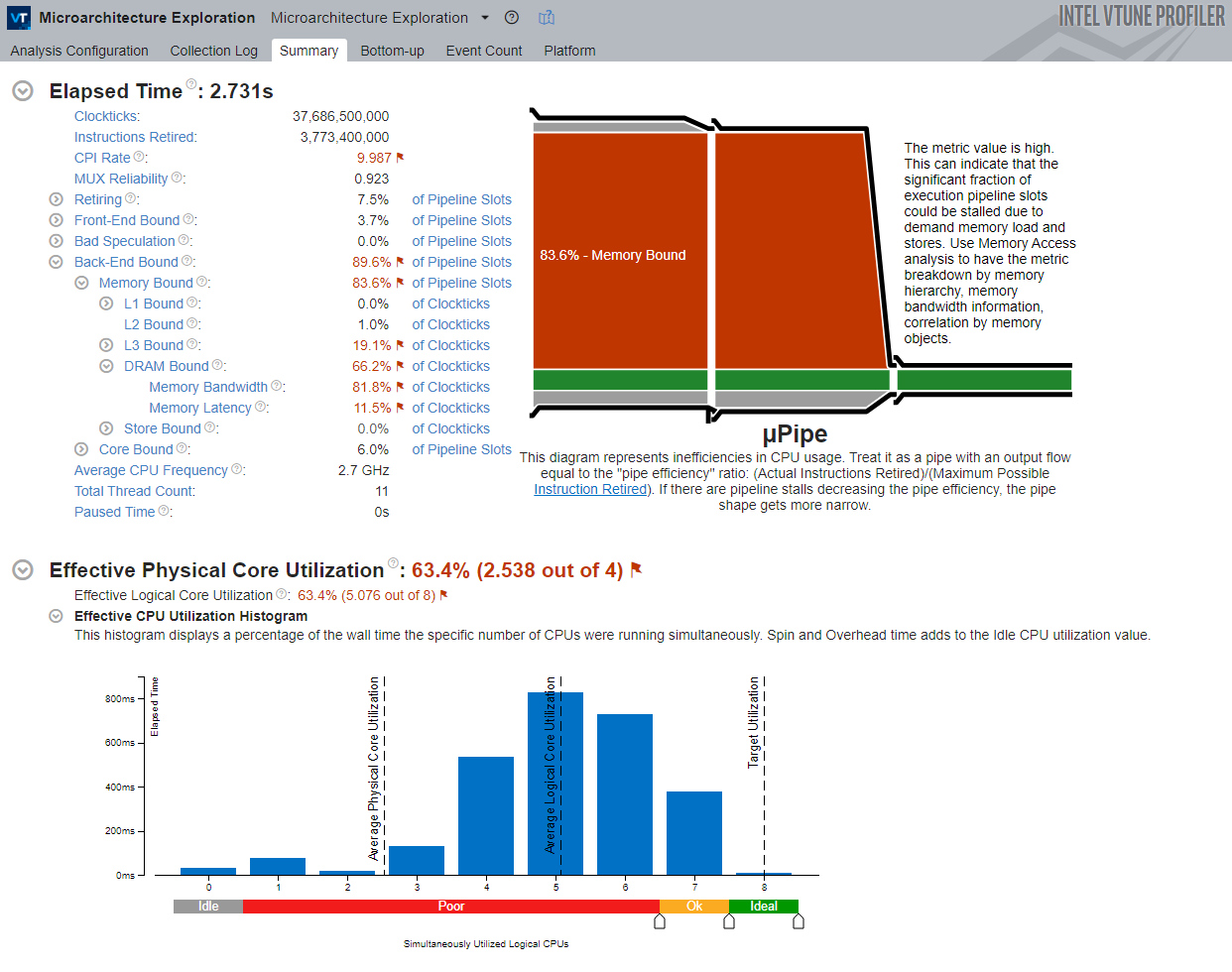
This view shows the following:

• Elapsed Time section: This section shows metrics related to the hardware utilization level. Hover over the marked metrics to see the problem description, possible causes, and suggestions for fixing the issue. The hierarchy of event-based metrics in the Microarchitecture Exploration view depends on your hardware architecture. Each metric is an event ratio defined by Intel architects and has its own predefined threshold. VTune evaluates the ratio value for each aggregated program unit, such as a function. When the value exceeds the threshold, it indicates a potential performance issue.
• µPipe Diagram: The μPipe, or microarchitecture pipeline, gives a graphical representation of CPU microarchitecture metrics and shows inefficient hardware usage. Think of it as a pipeline whose output throughput is equal to the ratio of actually retired instructions to the maximum possible retired instructions (pipeline efficiency). μPipe is based on CPU pipeline slots, which represent the hardware resources required to process one micro-op. Usually, multiple pipeline slots are available per cycle (pipeline width). If a pipeline slot does not retire, it is considered stalled, and the µPipe Diagram represents this as an obstacle that narrows the pipeline.
• Effective CPU Utilization Histogram: This histogram shows the elapsed time and usage level of the available logical processors and gives a graphical view of how many logical processors were used during application execution. Ideally, the tallest bar should match the target utilization level.

In this case, pay attention to the following metrics:

• The Memory Bound metric is high, so the application is constrained by memory access.
• The Memory Bandwidth and Memory Latency metrics are both high.

Taken together, these indicate a memory-access problem. However, this problem is slightly different in nature from the earlier one solved with loop interchange.

Before loop interchange was introduced, the application was mainly constrained by a cache-unfriendly memory-access pattern, which caused a large number of LLC (last-level cache) misses. That, in turn, led to frequent requests to DRAM.

Usually, most developers stop optimizing once the desired performance target is reached. The performance improvements obtained by optimizing the matrix application reduced wall time from about 90 seconds to about 2.5 seconds.

If you want to keep experimenting, you can modify the code to use cache blocking. Cache blocking is a way of reorganizing data access so that blocks of data are loaded into cache and reused when needed, greatly reducing the number of DRAM accesses.

To modify the code to use cache blocking, do the following:

In multiply.h, change line 36 as follows:

1- #define MULTIPLY multiply2
2+ #define MULTIPLY multiply4

Save the changes and rebuild the application.

This changes the code to use the multiply4 function in multiply.c, which implements cache blocking.

After rebuilding, you can run whichever analysis you choose to evaluate the performance improvement.

Visualizing the Performance Gain

VTune’s result-comparison feature can be used to better understand performance changes.

Although you can compare results from different analysis types, such as Hotspots and Performance Snapshot, only metrics that are available in both analysis types are shown.

To compare results:

1. Click the Compare Results button in the Main Toolbar.
2. Select the results you want to compare.

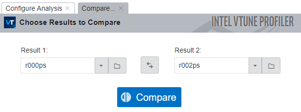
VTune computes the metric differences and opens the default Summary window:

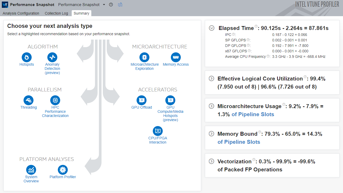
You can see that, for the matrix sample application, the runtime was reduced by nearly 88 seconds.

Notes

Click here to view